There was a damaging earthquake in Turkey yesterday, a magnitude M 6.1.
https://earthquake.usgs.gov/earthquakes/eventpage/us7000irp8/executive
The seismic hazards of this region of the Earth is dominated by a plate boundary fault, the North Anatolia fault (NAF).
The NAF is a right-lateral strike-slip earthquake fault that has a slip rate of about 24 mm/yr. This fault is similar in fault type and slip rate to the San Andreas fault in California.
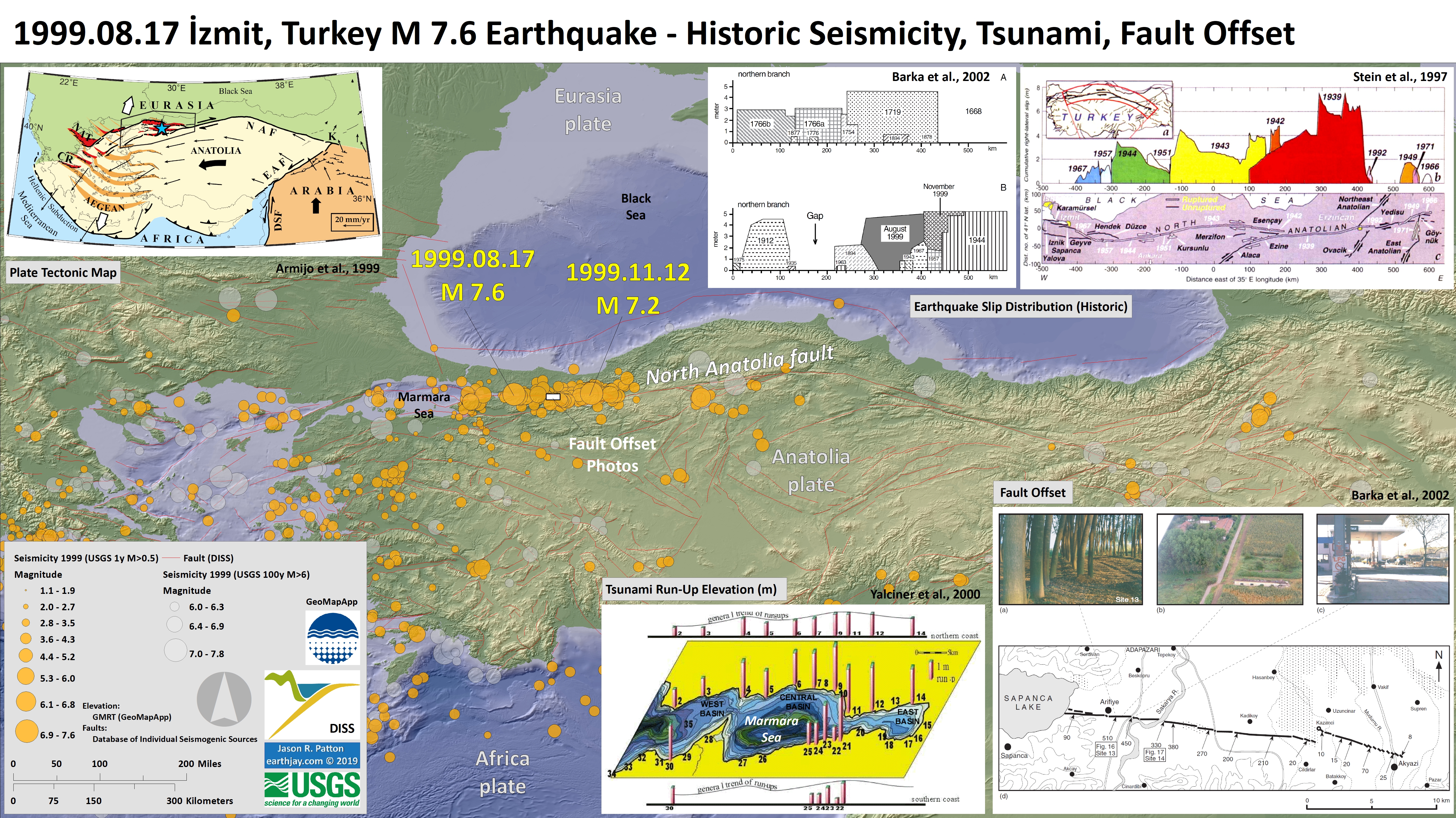
There have been a series of large earthquakes along the NAF in the 20th century. See the poster below that highlights the 1999 M 7.6 Izmit Earthquake.
Below is my interpretive poster for this earthquake
- I plot the seismicity from the past month, with diameter representing magnitude (see legend). I include earthquake epicenters from 1922-2022 with magnitudes M ≥ 3.0 in one version.
- I plot the USGS fault plane solutions (moment tensors in blue and focal mechanisms in orange), possibly in addition to some relevant historic earthquakes.
- A review of the basic base map variations and data that I use for the interpretive posters can be found on the Earthquake Reports page. I have improved these posters over time and some of this background information applies to the older posters.
- Some basic fundamentals of earthquake geology and plate tectonics can be found on the Earthquake Plate Tectonic Fundamentals page.
- In the upper left corner is a map that shows the tectonic strain in the region. Areas of red are deforming more from tectonic motion than are areas that are blue. Learn more about the Global Strain Rate Map project here.
- In the upper right corner is a comparison of the shaking intensity modeled by the USGS and the shaking intensity based on peoples’ “boots on the ground” observations. The closer to the earthquake, the stronger the ground shaking. A modeled estimate of intensity is shown by the color overlay and labels MMI 4, 5, 6, 7. The USGS Did You Feel It observations are the colored circles (color = intensity) and labeled dyfi 6.2 for example.
- Below the strain map is a plot that shows how the shaking intensity models and reports relate to each other. The horizontal axis is distance from the earthquake and the vertical axis is shaking intensity (using the MMI scale, just like in the map to the right: these are the same datasets).
- To the left of the intensity map is a tectonic map from Taymaz et al., 2007 that shows the main plate boundary faults and their relative senses of motion.
- To the left of the tectonic map is a plot from Stein et al. (1997) that shows the slip from these 20th century earthquakes along the NAF.
- To the left of the Stein figure are two histograms from the USGS PAGER Alert system. These are rapid estimates of the potential damage from this earthquake. These data help organizations understand what response programs need to be utilized to help the people in this region following this earthquake.
- In the center right is a map from the Seismic Hazard Harmonization in Europe program, which shows the chance for ground shaking from earthquakes over the next 50 years.
- In the lower right corner is a larger scale map showing the tectonic geomorphology of the region (how the landscape is sculpted by tectonic forces). This map has aftershocks from the CSEM-EMSC catalog.
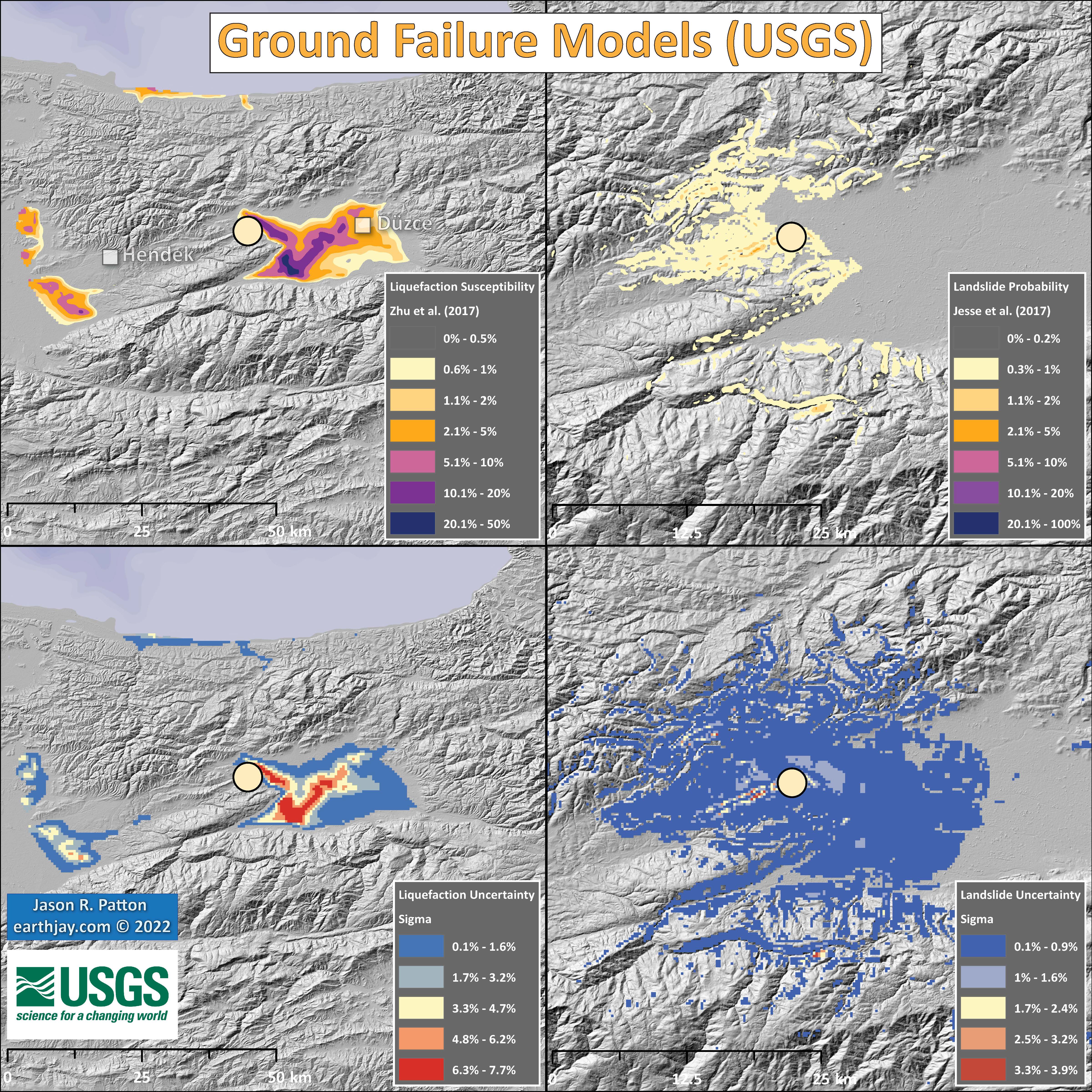
- To the right of the legend are two maps that show (left) liquefaction susceptibility and (right) landslide probability. These are based on empirical models from the USGS that show the chance an area may have experienced these processes that may have happened as a result of the ground shaking from the earthquake. I spend more time explaining these types of models and what they represent in this Earthquake Report for the recent event in Albania.
I include some inset figures. Some of the same figures are located in different places on the larger scale map below.
- Here is the map with 3 month’s seismicity plotted.

Other Report Pages
Some Relevant Discussion and Figures
- This is the plate tectonic map from Armijo et al., 1999.
Tectonic setting of continental extrusion in eastern Mediterranean. Anatolia-Aegean block escapes westward from Arabia-Eurasia collision zone, toward Hellenic subduction zone. Current motion relative to Eurasia (GPS [Global Positioning System] and SLR [Satellite Laser Ranging] velocity vectors, in mm/yr, from Reilinger et al., 1997). In Aegean, two deformation regimes are superimposed (Armijo et al., 1996): widespread, slow extension starting earlier (orange stripes, white diverging arrows), and more localized, fast transtension associated with later, westward propagation of North Anatolian fault (NAF). EAF—East Anatolian fault, K—Karliova triple junction, DSF—Dead Sea fault,NAT—North Aegean Trough, CR—Corinth Rift.Box outlines Marmara pull-apart region, where North Anatolian fault enters Aegean.
- Here is the tectonic map from Dilek and Sandvol (2009).
Tectonic map of the Aegean and eastern Mediterranean region showing the main plate boundaries, major suture zones, fault systems and tectonic units. Thick, white arrows depict the direction and magnitude (mm a21) of plate convergence; grey arrows mark the direction of extension (Miocene–Recent). Orange and purple delineate Eurasian and African plate affinities, respectively. Key to lettering: BF, Burdur fault; CACC, Central Anatolian Crystalline Complex; DKF, Datc¸a–Kale fault (part of the SW Anatolian Shear Zone); EAFZ, East Anatolian fault zone; EF, Ecemis fault; EKP, Erzurum–Kars Plateau; IASZ, Izmir–Ankara suture zone; IPS, Intra–Pontide suture zone; ITS, Inner–Tauride suture; KF, Kefalonia fault; KOTJ, Karliova triple junction; MM, Menderes massif; MS, Marmara Sea; MTR, Maras triple junction; NAFZ, North Anatolian fault zone; OF, Ovacik fault; PSF, Pampak–Sevan fault; TF, Tutak fault; TGF, Tuzgo¨lu¨ fault; TIP, Turkish–Iranian plateau (modified from Dilek 2006).
- This is the Woudloper (2009) tectonic map of the Mediterranean Sea. The yellow/orange band represents the Alpide Belt, a convergent plate boundary that extends from western Europe, through the Middle East, beneath northern India and Nepal (forming the Himalayas), through Indonesia, terminating east of Australia.
- This is a fantastic figure, yet quite complicated. This map shows teh plate boundaries, the GPS motions, and the tectonic strain for the region (Perouse et al., 2012).
- We use GPS sites at specific locations to measure how fast the Earth’s crust moves due to plate tectonics and other reasons. These GPS sites are almost constantly recording their geographic position. If a GPS site is moving, we can take two observations (lets say a year apart), measure their relative distance, and divide the time between the measurements to get the velocity (the speed) that this GPS site is moving. The white vectors (the arrows) show the direction those GPS sites are moving and the length of the vector represents its velocity. The black arrows show what the plate motion rates are at the plate boundaries and these are modeled using lots of different data sources (not just GPS).
- Tectonic strain is a measure of how much the Earth’s crust is deforming over time. The higher the tectonic strain rate (i.e. red), the more tectonic stress is being accumulated in the crust and along faults. Areas of higher strain are places where there are more likely to be larger or more (or both) earthquakes.
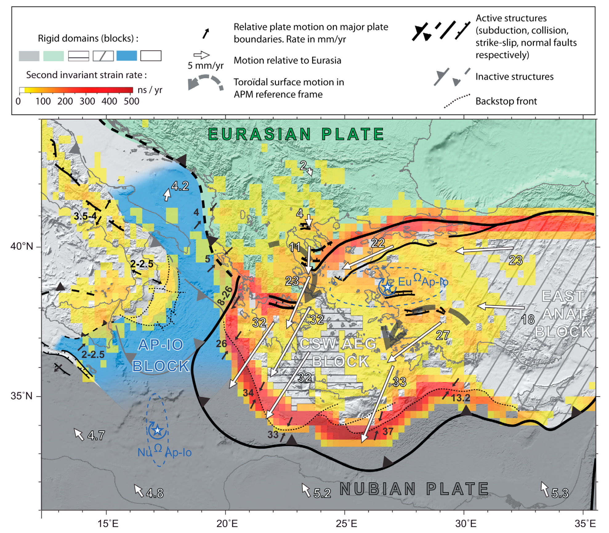
Present-day kinematic and tectonic map encompassing the Central and Eastern Mediterranean, summarizing our main results and interpretations. Our kinematic model includes rigid-block motions as well as localized and distributed strain. Central-SW Aegean block (CSW AEG block) and East Anatolian block (East Anat. block) are purely kinematic and directly results from strain modeling (Figure 5). AP-IO Block is our Apulian-Ionian block with tentative tectonic boundaries. Rotation pole of this Apulian-Ionian block relative to Nubia (Nu WAp-Io) and to Eurasia (Eu WAp-Io) are shown with their 95% confidence ellipse.
- Below is a series of figures from Jolivet et al. (2013). These show various data sets and analyses for Greece and Turkey.
- Upper Panel (A): This is a tectonic map showing the major faults and geologic terranes in the region. The fault possibly associated with today’s earthquake is labeled “Neo Tethys Suture” on the map, for the Eastern Anatolia fault.
- Lower Panel (B): This shows historic seismicity for the region. Note the general correlation with the faults in the upper panel.
- Upper Panel (C): These red arrows are Global Positioning System (GPS) velocity vectors. The velocity scale vector is in the lower left corner. The main geodetic (study of plate motions and deformation of the earth) signal here is the westward motion of the North Anatolian fault system as it rotates southward as it traverses Greece. The motion trends almost south near the island of Crete, which is perpendicular to the subduction zone.
- Lower Panel (D): This map shows the region of mid-Cenozoic (Oligo-Miocene) extension (shaded orange). It just happens that there is still extension going on in parts of this prehistoric extension.
- Upper Panel (E): This map shows where the downgoing slab may be located (in blue), along with the volcanic centers associated with the subduction zone in the past.
- Lower Panel (F): This map shows the orientation of how seismic waves orient themselves differently in different places (anisotropy). We think seismic waves travel in ways that reflects how tectonic strain is stored in the earth. The blue lines show the direction of extension in the asthenosphere, green lines in the lithospheric mantle, and red lines for the crust.
- Upper Panel (G): This is the map showing focal mechanisms in the poster above. Note the strike slip earthquakes associated with the North Anatolia and East Anatolia faults and the thrust/reverse mechanisms associated with the thrust faults.
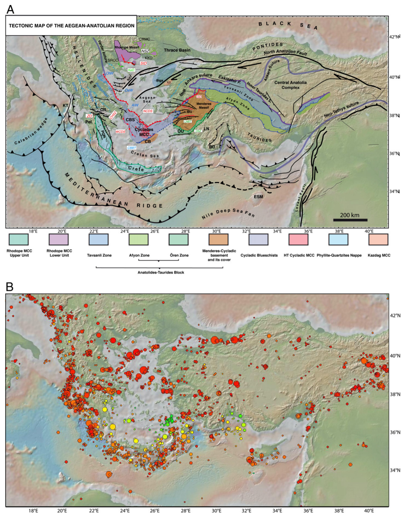
A: Tectonic map of the Aegean and Anatolian region showing the main active structures
(black lines), the main sutures zones (thick violet or blue lines), the main thrusts in the Hellenides where they have not been reworked by later extension (thin blue lines), the North Cycladic Detachment (NCDS, in red) and its extension in the Simav Detachment (SD), the main metamorphic units and their contacts; AlW: Almyropotamos window; BD: Bey Daglari; CB: Cycladic Basement; CBBT: Cycladic Basement basal thrust; CBS: Cycladic Blueschists; CHSZ: Central Hellenic Shear Zone; CR: Corinth Rift; CRMC: Central Rhodope Metamorphic Complex; GT: Gavrovo–Tripolitza Nappe; KD: Kazdag dome; KeD: Kerdylion Detachment; KKD: Kesebir–Kardamos dome; KT: Kephalonia Transform Fault; LN: Lycian Nappes; LNBT: Lycian Nappes Basal Thrust; MCC: Metamorphic Core Complex; MG: Menderes Grabens; NAT: North Aegean Trough; NCDS: North Cycladic Detachment System; NSZ: Nestos Shear Zone; OlW: Olympos Window; OsW: Ossa Window; OSZ: Ören Shear Zone; Pel.: Peloponnese; ÖU: Ören Unit; PQN: Phyllite–Quartzite Nappe; SiD: Simav Detachment; SRCC: South Rhodope Core Complex; StD: Strymon Detachment; WCDS: West Cycladic Detachment System; ZD: Zaroukla Detachment. B: Seismicity. Earthquakes are taken from the USGS-NEIC database. Colour of symbols gives the depth (blue for shallow depths) and size gives the magnitude (from 4.5 to 7.6).
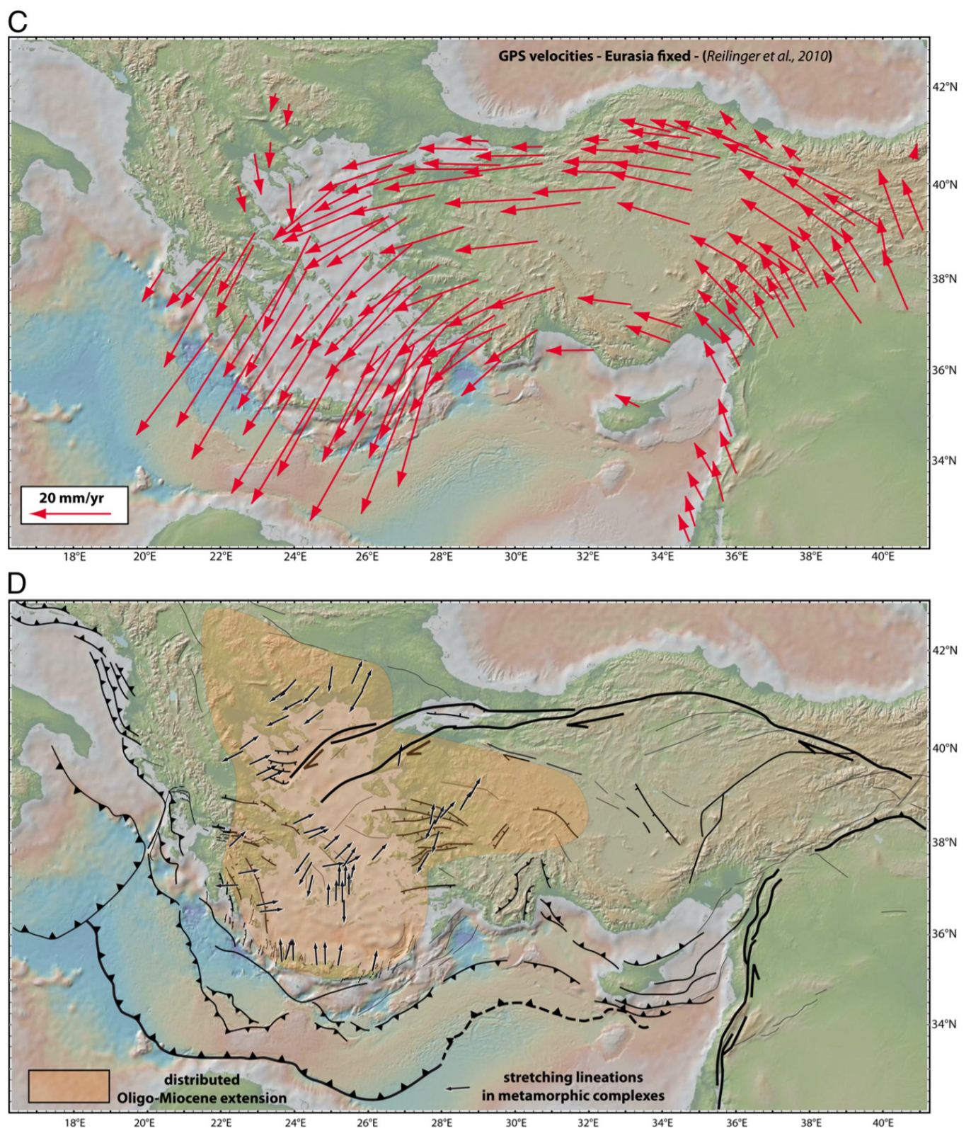
C: GPS velocity field with a fixed Eurasia after Reilinger et al. (2010) D: the domain affected by distributed post-orogenic extension in the Oligocene and the Miocene and the stretching lineations in the exhumed metamorphic complexes.
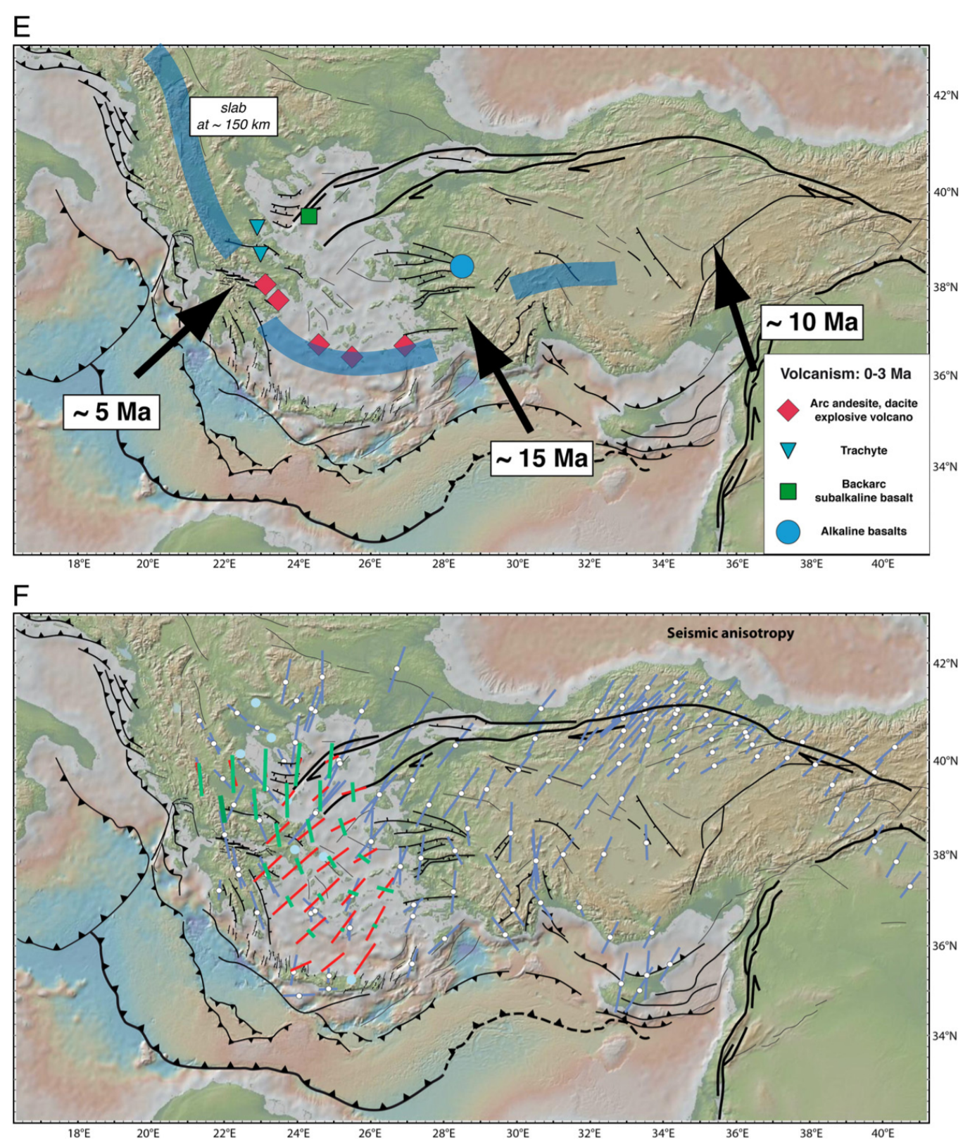
E: The thick blue lines illustrate the schematized position of the slab at ~150 km according to the tomographic model of Piromallo and Morelli (2003), and show the disruption of the slab at three positions and possible ages of these tears discussed in the text. Velocity anomalies are displayed in percentages with respect to the reference model sp6 (Morelli and Dziewonski, 1993). Coloured symbols represent the volcanic centres between 0 and 3 Ma after Pe-Piper and Piper (2006). F: Seismic anisotropy obtained from SKS waves (blue bars, Paul et al., 2010) and Rayleigh waves (green and orange bars, Endrun et al., 2011). See also Sandvol et al. (2003). Blue lines show the direction of stretching in the asthenosphere, green bars represent the stretching in the lithospheric mantle and orange bars in the lower crust.
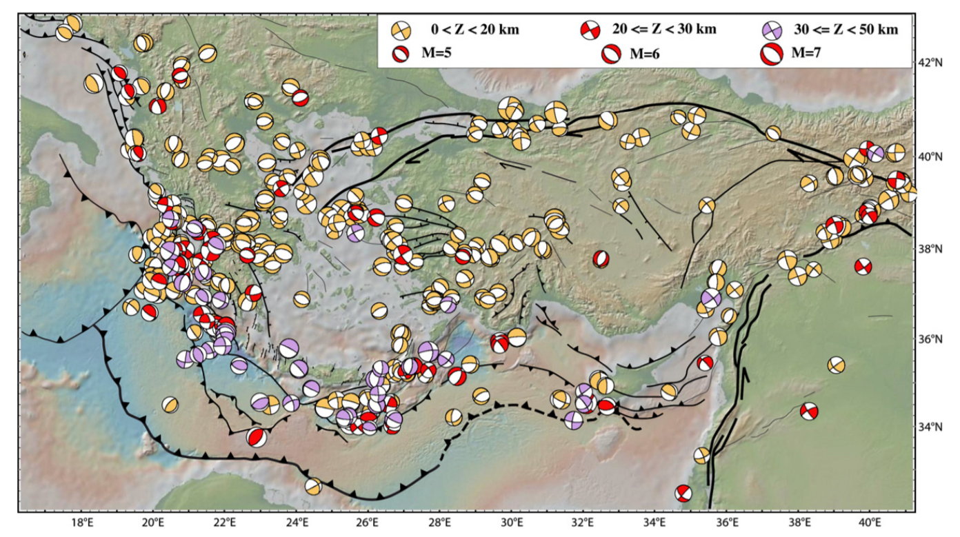
G: Focal mechanisms of earthquakes over the Aegean Anatolian region.
- Here is a map showing tectonic domains (Taymaz et al., 2007).

Schematic map of the principal tectonic settings in the Eastern Mediterranean. Hatching shows areas of coherent motion and zones of distributed deformation. Large arrows designate generalized regional motion (in mm a21) and errors (recompiled after McClusky et al. (2000, 2003). NAF, North Anatolian Fault; EAF, East Anatolian Fault; DSF, Dead Sea Fault; NEAF, North East Anatolian Fault; EPF, Ezinepazarı Fault; CTF, Cephalonia Transform Fault; PTF, Paphos Transform Fault.
- Because this 1999 earthquake is important for many reasons, I will be writing up an Earthquake Report for that event sometime soon. In the meantime, here is a poster I put together for that event.
- Of particular note is that this August earthquake generated a small tsunami. I use this in my tsunami talks to highlight how there are non-traditional tsunami sources that need to be considered when mitigating tsunami hazards. Even though this tsunami was only a couple meters high, that is enough to damage harbors, boats, and people.
- There are many different ways in which a landslide can be triggered. The first order relations behind slope failure (landslides) is that the “resisting” forces that are preventing slope failure (e.g. the strength of the bedrock or soil) are overcome by the “driving” forces that are pushing this land downwards (e.g. gravity). The ratio of resisting forces to driving forces is called the Factor of Safety (FOS). We can write this ratio like this:
FOS = Resisting Force / Driving Force
- When FOS > 1, the slope is stable and when FOS < 1, the slope fails and we get a landslide. The illustration below shows these relations. Note how the slope angle α can take part in this ratio (the steeper the slope, the greater impact of the mass of the slope can contribute to driving forces). The real world is more complicated than the simplified illustration below.
- Landslide ground shaking can change the Factor of Safety in several ways that might increase the driving force or decrease the resisting force. Keefer (1984) studied a global data set of earthquake triggered landslides and found that larger earthquakes trigger larger and more numerous landslides across a larger area than do smaller earthquakes. Earthquakes can cause landslides because the seismic waves can cause the driving force to increase (the earthquake motions can “push” the land downwards), leading to a landslide. In addition, ground shaking can change the strength of these earth materials (a form of resisting force) with a process called liquefaction.
- Sediment or soil strength is based upon the ability for sediment particles to push against each other without moving. This is a combination of friction and the forces exerted between these particles. This is loosely what we call the “angle of internal friction.” Liquefaction is a process by which pore pressure increases cause water to push out against the sediment particles so that they are no longer touching.
- An analogy that some may be familiar with relates to a visit to the beach. When one is walking on the wet sand near the shoreline, the sand may hold the weight of our body generally pretty well. However, if we stop and vibrate our feet back and forth, this causes pore pressure to increase and we sink into the sand as the sand liquefies. Or, at least our feet sink into the sand.
- Below is a diagram showing how an increase in pore pressure can push against the sediment particles so that they are not touching any more. This allows the particles to move around and this is why our feet sink in the sand in the analogy above. This is also what changes the strength of earth materials such that a landslide can be triggered.
- Below is a diagram based upon a publication designed to educate the public about landslides and the processes that trigger them (USGS, 2004). Additional background information about landslide types can be found in Highland et al. (2008). There was a variety of landslide types that can be observed surrounding the earthquake region. So, this illustration can help people when they observing the landscape response to the earthquake whether they are using aerial imagery, photos in newspaper or website articles, or videos on social media. Will you be able to locate a landslide scarp or the toe of a landslide? This figure shows a rotational landslide, one where the land rotates along a curvilinear failure surface.
- Here is an excellent educational video from IRIS and a variety of organizations. The video helps us learn about how earthquake intensity gets smaller with distance from an earthquake. The concept of liquefaction is reviewed and we learn how different types of bedrock and underlying earth materials can affect the severity of ground shaking in a given location. The intensity map above is based on a model that relates intensity with distance to the earthquake, but does not incorporate changes in material properties as the video below mentions is an important factor that can increase intensity in places.
- If we look at the map at the top of this report, we might imagine that because the areas close to the fault shake more strongly, there may be more landslides in those areas. This is probably true at first order, but the variation in material properties and water content also control where landslides might occur.
- There are landslide slope stability and liquefaction susceptibility models based on empirical data from past earthquakes. The USGS has recently incorporated these types of analyses into their earthquake event pages. More about these USGS models can be found on this page.
- Below is a figure that shows both landslide probability and liquefaction susceptibility maps for this M 6.1 earthquake.
- For the first time, I include maps that show the uncertainty in these ground failure models. The larger the uncertainty is shown in red and the lower the uncertainty is shown in blue. I cut off the symbology at 0.1%.
Earthquake Triggered Landslides


Seismic Hazard and Seismic Risk
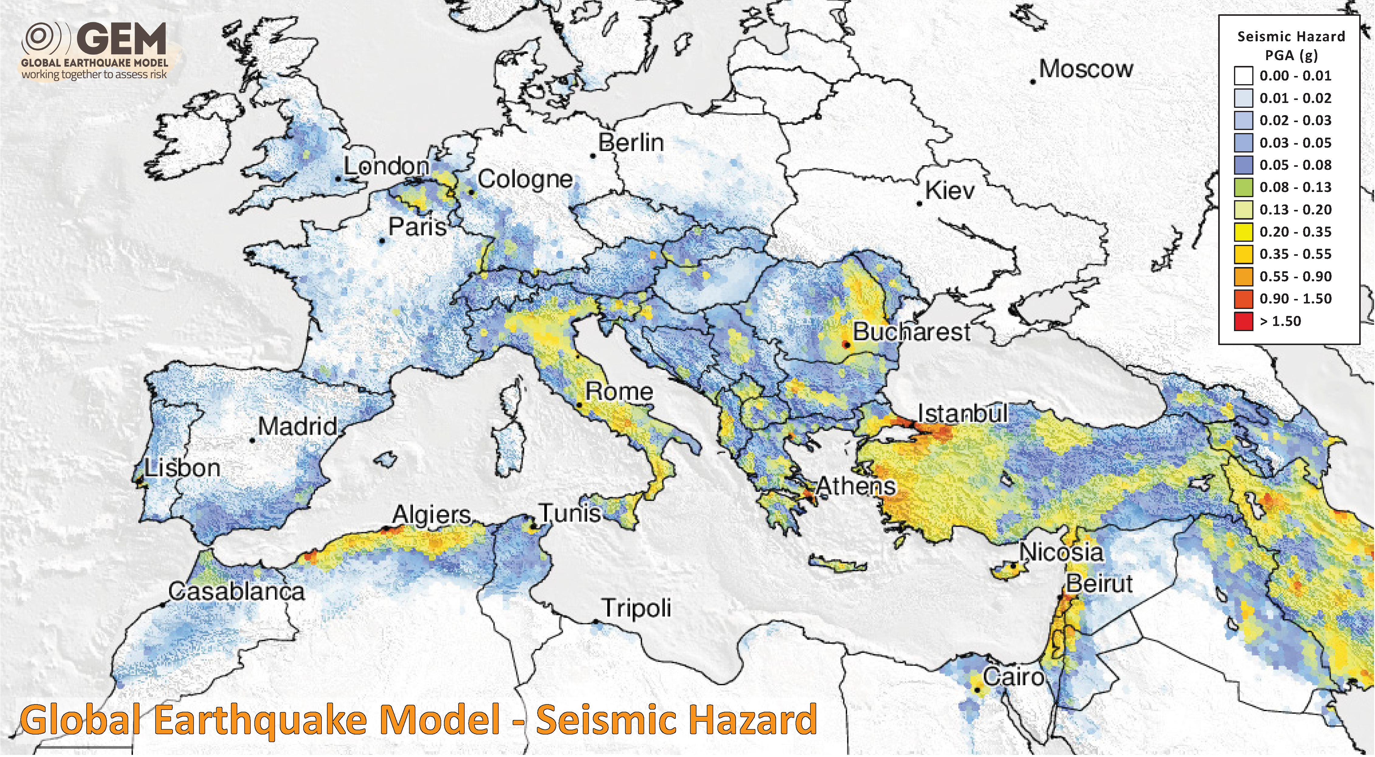
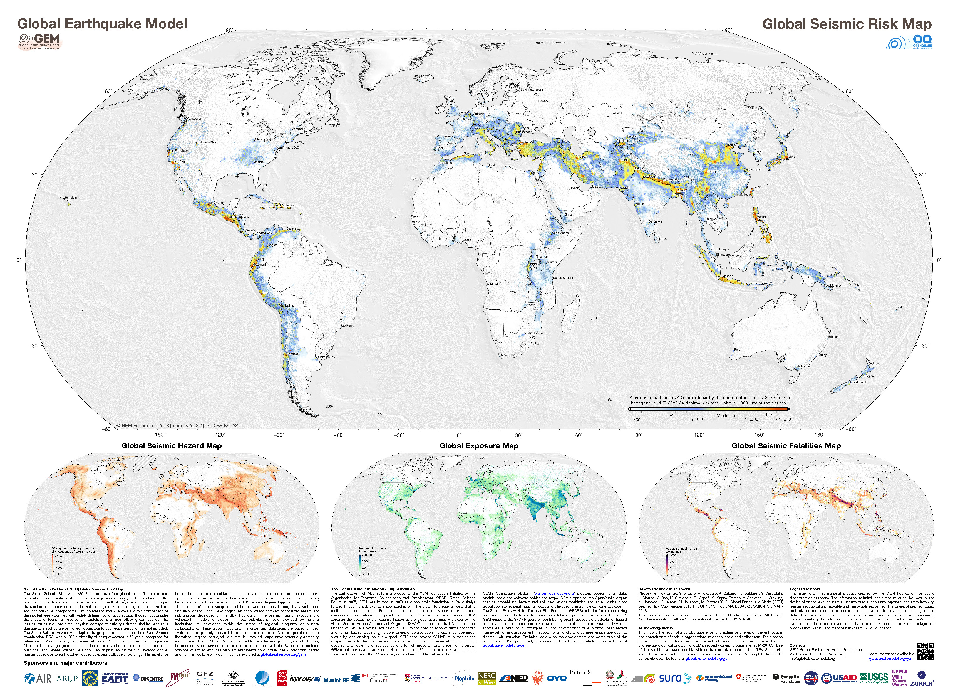
- These are the two seismic maps from the Global Earthquake Model (GEM) project, the GEM Seismic Hazard and the GEM Seismic Risk maps from Pagani et al. (2018) and Silva et al. (2018).
- The GEM Seismic Hazard Map:
- The Global Earthquake Model (GEM) Global Seismic Hazard Map (version 2018.1) depicts the geographic distribution of the Peak Ground Acceleration (PGA) with a 10% probability of being exceeded in 50 years, computed for reference rock conditions (shear wave velocity, VS30, of 760-800 m/s). The map was created by collating maps computed using national and regional probabilistic seismic hazard models developed by various institutions and projects, and by GEM Foundation scientists. The OpenQuake engine, an open-source seismic hazard and risk calculation software developed principally by the GEM Foundation, was used to calculate the hazard values. A smoothing methodology was applied to homogenise hazard values along the model borders. The map is based on a database of hazard models described using the OpenQuake engine data format (NRML). Due to possible model limitations, regions portrayed with low hazard may still experience potentially damaging earthquakes.
- Here is a view of the GEM seismic hazard map for Europe.
- The USGS Seismic Hazard Map:
- Here is a map that displays an estimate of seismic hazard for the region (Jenkins et al., 2010). This comes from Giardini et al. (1999).
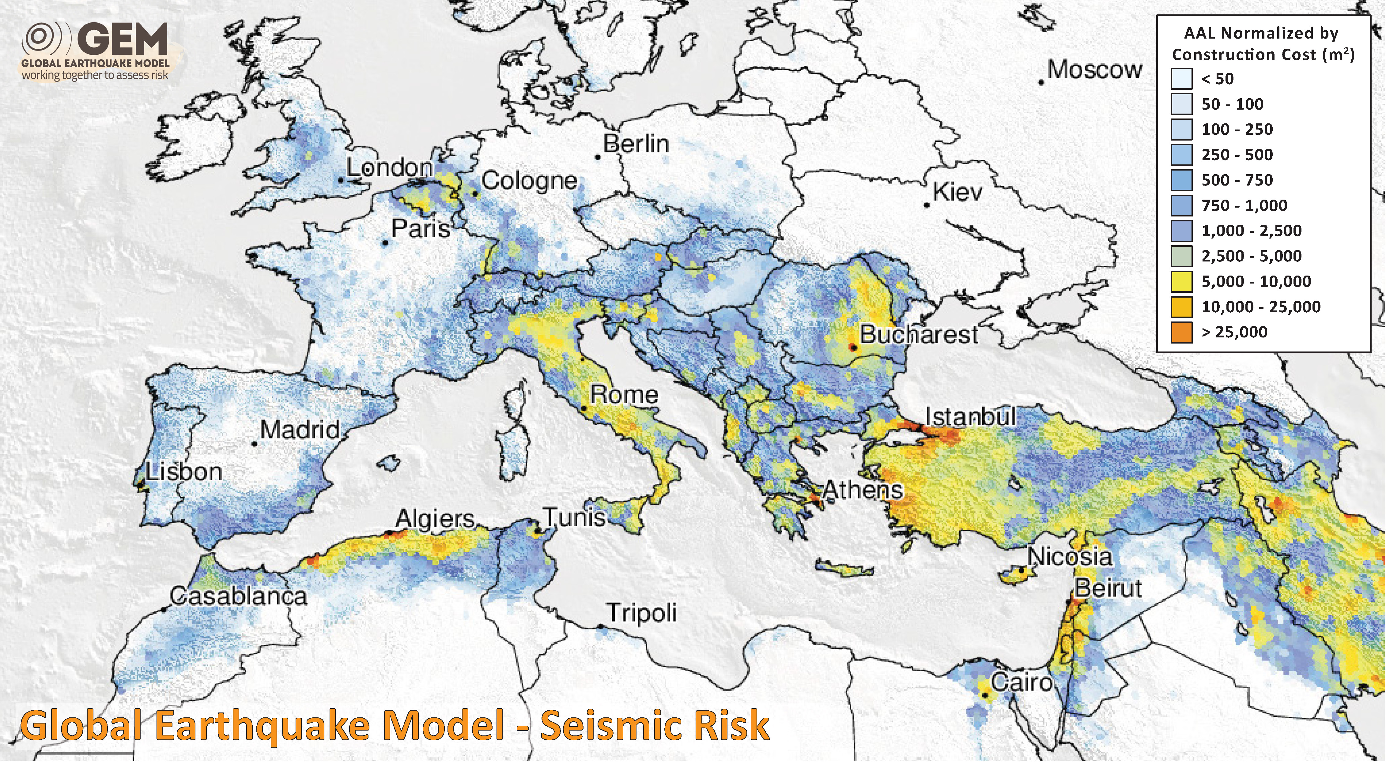
- The GEM Seismic Risk Map:
- The Global Seismic Risk Map (v2018.1) presents the geographic distribution of average annual loss (USD) normalised by the average construction costs of the respective country (USD/m2) due to ground shaking in the residential, commercial and industrial building stock, considering contents, structural and non-structural components. The normalised metric allows a direct comparison of the risk between countries with widely different construction costs. It does not consider the effects of tsunamis, liquefaction, landslides, and fires following earthquakes. The loss estimates are from direct physical damage to buildings due to shaking, and thus damage to infrastructure or indirect losses due to business interruption are not included. The average annual losses are presented on a hexagonal grid, with a spacing of 0.30 x 0.34 decimal degrees (approximately 1,000 km2 at the equator). The average annual losses were computed using the event-based calculator of the OpenQuake engine, an open-source software for seismic hazard and risk analysis developed by the GEM Foundation. The seismic hazard, exposure and vulnerability models employed in these calculations were provided by national institutions, or developed within the scope of regional programs or bilateral collaborations.
- Here is a view of the GEM seismic risk map for Europe.
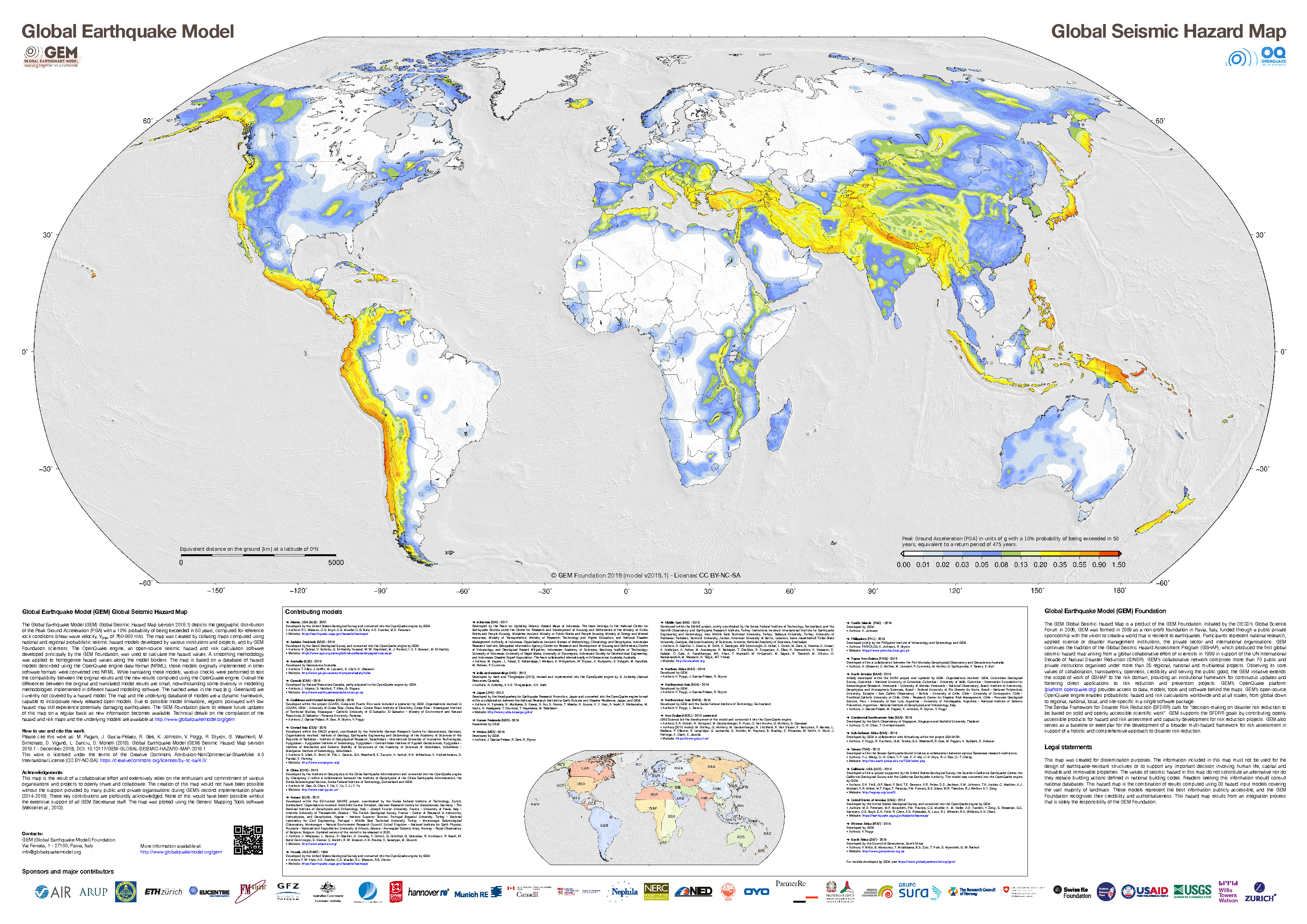
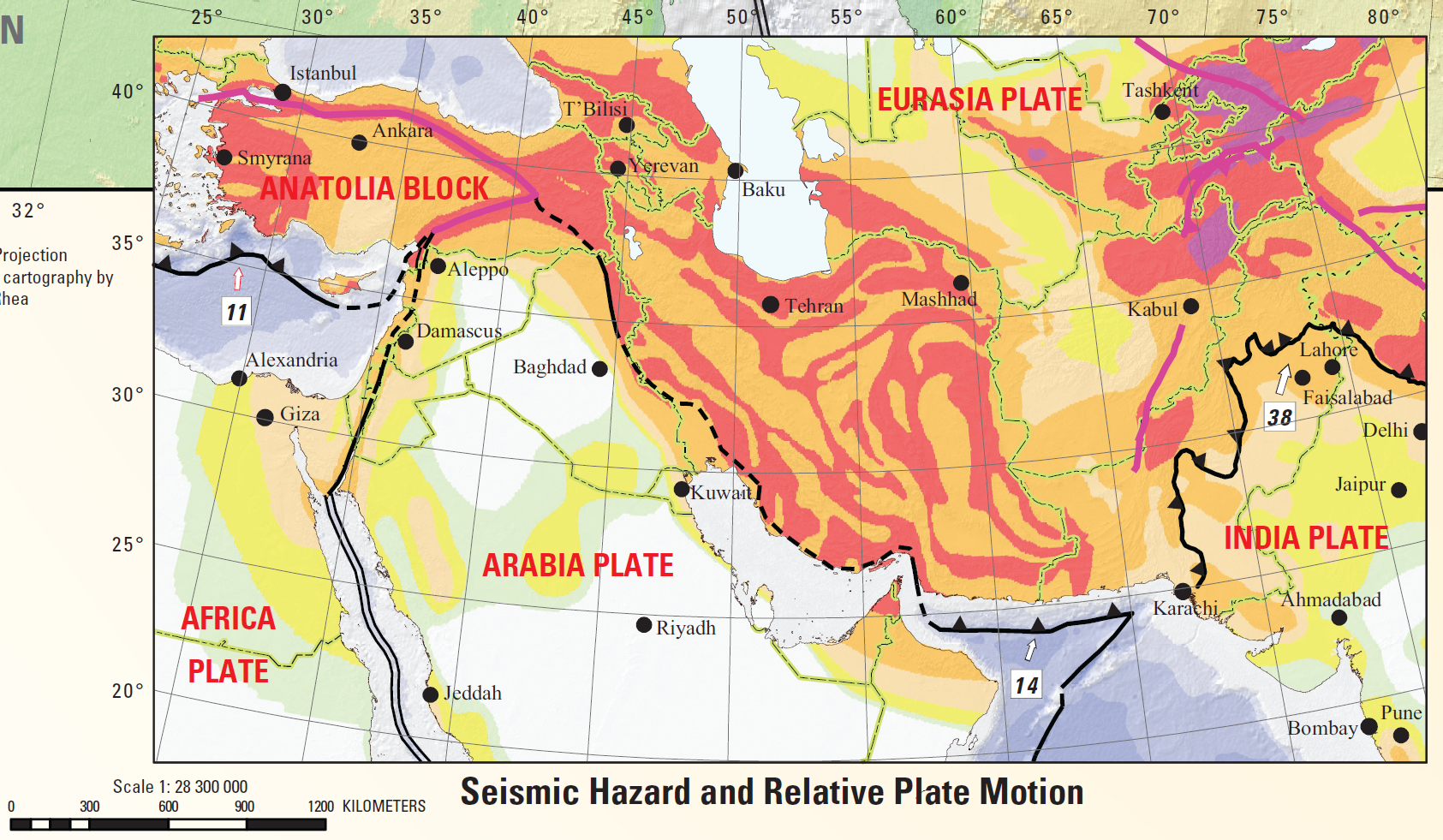
The Global Seismic Hazard Map. Peak ground acceleration (pga) with a 10% chance of exceedance in 50 years is depicted in m/s2. The site classification is rock everywhere except Canada and the United States, which assume rock/firm soil site classifications. White and green correspond to low seismicity hazard (0%-8%g), yellow and orange correspond to moderate seismic hazard (8%-24%g), pink and dark pink correspond to high seismicity hazard (24%-40%g), and red and brown correspond to very high seismic hazard (greater than 40%g).
- 2022.11.23 M 6.1 Turkey
- 2020.12.30 M 6.4 Croatia
- 2020.10.30 M 7.0 Turkey
- 2020.05.02 M 6.6 Crete, Greece
- 2020.01.24 M 6.7 Turkey
- 2019.11.26 M 6.4 Albania
- 2018.10.25 M 6.8 Greece
- 2017.07.20 M 6.7 Turkey
- 2017.06.12 M 6.3 Turkey/Greece
- 2016.10.30 M 6.6 Italy
- 2016.10.30 M 6.6 Italy Update #1
- 2016.10.28 M 5.8 Tyrrhenian Sea
- 2016.10.26 M 6.1 Italy
- 2016.10.16 M 5.3 Greece/Albania
- 2016.08.23 M 6.2 Italy
- 2016.01.24 M 6.1 Mediterranean
- 2015.11.17 M 6.5 Greece
- 2015.04.16 M 6.0 Crete
Europe
General Overview
Earthquake Reports
Social Media
#EarthquakeReport for M6.1 #Deprem #Earthquake in northern #Turkey
probably a right-lateral strike-slip earthquake along the North Anatolia fault system
strong shaking in the Düzce region, close to the 1999 M7.2 temblor
read more in the report herehttps://t.co/7rNAKb3zJu pic.twitter.com/juJlK2L1WM
— Jason "Jay" R. Patton (@patton_cascadia) November 24, 2022
Early morning, Nov. 23 local time, a magnitude 6.1 earthquake occurred 16 km (10 mi) west of Düzce, Turkey. This event is currently at PAGER level orange, indicating significant damage is likely & the disaster is potentially widespread. Our thoughts are with the people of Düzce. https://t.co/0fRUHHnnaS pic.twitter.com/CG2DuWfOfK
— USGS Earthquakes (@USGS_Quakes) November 23, 2022
⚠️ Confirmed: Real-time network data show a significant disruption to internet connectivity in #Düzce, #Turkey following a 5.9 magnitude earthquake; the outages are attributed to widespread power cuts reported in the region 📉 pic.twitter.com/88Wi87Am4i
— NetBlocks (@netblocks) November 23, 2022
Also playing in to this is the Baader-Meinhof phenomenon, also known as the frequency illusion. https://t.co/yWLqZIoN8b
— Wendy Bohon, PhD 🌏 (@DrWendyRocks) November 23, 2022
The region has already a lot of landslides. Triggering will depend on H2O saturation. The NAF also created quite a lot of pull apart basins which are prone to liquefaction, especially around Golyaka
— Oz ⚒️ (@OzgurKozaci) November 23, 2022
It looks like side faulde of main North Anatolian Fault
At 11/1999 we had major earthquake (7.2Mw) on the NAF segment
08/1999 (7.6Mw) Marmara earthquake had struck southern bold red higlihted faultToday's tremble was felt over a vast area from western istanbul to ankara pic.twitter.com/RUaU9qKLus
— Emre Evren (@EmreEvren_IYI) November 23, 2022
#Latest 5.9 Mw (#KRDAE) Northern #TURKEY 🇹🇷, a shallow right-lateral strike-slip (Karadere-Düzce Branch/North Anatolian Fault System), possible severe damage in nearby localities, figure from Roux/Ben-Zion et al. 2014. pic.twitter.com/0JGFmoKgfa
— Abel Seism🌏Sánchez (@EQuake_Analysis) November 23, 2022
Mw=6.1, TURKEY (Depth: 12 km), 2022/11/23 01:08:14 UTC – Full details here: https://t.co/IMFvc2js15 pic.twitter.com/PJ2MJMlpKS
— Earthquakes (@geoscope_ipgp) November 23, 2022
Düzce'de #deprem anı… pic.twitter.com/zfjsy7j17T
— İzzet Altaş (@izzetaltas_) November 23, 2022
Updated source mechanism of 2022.11.23 Mw6.0 Düzce Earthquake. Green lines=Broken parts of the NAF(Konca et al., 2010; Bouchon et al., 2002). Red line=Unbroken part of Karadere Segment. LowerPanel:Coulomb stress change (Location:@Kandilli_info) pic.twitter.com/GthYfz9ElY
— Sezim (@sezim_guvercin) November 23, 2022
In 1999 the North Anatolian Fault (NAF), broke during two destructive #earthquakes (Mw7.4 Izmit and Mw7.2 Düzce). Today's Mw6.1 #earthquake happened east of Düzce with mechanism similar to 2019 event.
Mechanism https://t.co/dKXlLfRKkt
and 1999 rupture map https://t.co/rWvuOEAIPo pic.twitter.com/sSyFd5SmGj— Robin Lacassin – @RobinLacassin@qoto.org (@RLacassin) November 23, 2022
Manually revised solution FMNEAR (Géoazur/OCA) with regional records for the M 6.1 – WESTERN TURKEY – 2022-11-23 01:08:15 UTC (Loc KOERI used).https://t.co/UHDsc1hVXA
Thanks to the seismic records provided in particular by KOERI and IRIS pic.twitter.com/3unR3l5aAZ
— Bertrand Delouis (@BertrandDelouis) November 23, 2022
📌 A brief information about Gölyaka (Düzce) Earthquake (Mw=5.9)
Date: 23.11.2022
Time: 04:08 (Local Time)#Earthquake #Duzceearthquake@LastQuake @ISCseism pic.twitter.com/T5xXRqpnIH— AFAD Deprem (@DepremDairesi) November 23, 2022
Düzce de bir iş yerinin güvenlik kamerasına yansıyam görüntüler çok korkunç rabbim beterinden korusun #deprem pic.twitter.com/Qm7zgygaY1
— Ozan Aydoğdu (@OzyAydogdu) November 23, 2022
23 Kasım 2022 #Düzce-Gölyaka depreminin (Mw=6.0) 230km uzaklıktaki Marmara Denizi'nde 23yıl geçmesine karşın, henüz gerçekleşmeyen beklenen olası #deprem'i etkilemesi söz konusu değildir. Böyle bir bağlantı kurabilecek/ispatlayacak bölgesel bir stres haritası bile sunamazsınız. pic.twitter.com/yWAC3uKHjS
— Dr. Ramazan Demirtaş (@Paleosismolog) November 23, 2022
Interesting @NERC_COMET 2020 webinar from Dr Jonathan Weiss & Dr Chris Rollins.
Great use of @CopernicusEU #Sentinel1 to help resolve strain rate, & earthquake hazards, in Anatolia. Shows why Mag 5.9 earthquakes, like Duzce, should come as no surprise.https://t.co/UaobvrrHXS pic.twitter.com/jyCFstX9rX
— DPManchee (@DPManchee) November 24, 2022
- Frisch, W., Meschede, M., Blakey, R., 2011. Plate Tectonics, Springer-Verlag, London, 213 pp.
- Hayes, G., 2018, Slab2 – A Comprehensive Subduction Zone Geometry Model: U.S. Geological Survey data release, https://doi.org/10.5066/F7PV6JNV.
- Holt, W. E., C. Kreemer, A. J. Haines, L. Estey, C. Meertens, G. Blewitt, and D. Lavallee (2005), Project helps constrain continental dynamics and seismic hazards, Eos Trans. AGU, 86(41), 383–387, , https://doi.org/10.1029/2005EO410002. /li>
- Jessee, M.A.N., Hamburger, M. W., Allstadt, K., Wald, D. J., Robeson, S. M., Tanyas, H., et al. (2018). A global empirical model for near-real-time assessment of seismically induced landslides. Journal of Geophysical Research: Earth Surface, 123, 1835–1859. https://doi.org/10.1029/2017JF004494
- Kreemer, C., J. Haines, W. Holt, G. Blewitt, and D. Lavallee (2000), On the determination of a global strain rate model, Geophys. J. Int., 52(10), 765–770.
- Kreemer, C., W. E. Holt, and A. J. Haines (2003), An integrated global model of present-day plate motions and plate boundary deformation, Geophys. J. Int., 154(1), 8–34, , https://doi.org/10.1046/j.1365-246X.2003.01917.x.
- Kreemer, C., G. Blewitt, E.C. Klein, 2014. A geodetic plate motion and Global Strain Rate Model in Geochemistry, Geophysics, Geosystems, v. 15, p. 3849-3889, https://doi.org/10.1002/2014GC005407.
- Meyer, B., Saltus, R., Chulliat, a., 2017. EMAG2: Earth Magnetic Anomaly Grid (2-arc-minute resolution) Version 3. National Centers for Environmental Information, NOAA. Model. https://doi.org/10.7289/V5H70CVX
- Müller, R.D., Sdrolias, M., Gaina, C. and Roest, W.R., 2008, Age spreading rates and spreading asymmetry of the world’s ocean crust in Geochemistry, Geophysics, Geosystems, 9, Q04006, https://doi.org/10.1029/2007GC001743
- Pagani,M. , J. Garcia-Pelaez, R. Gee, K. Johnson, V. Poggi, R. Styron, G. Weatherill, M. Simionato, D. Viganò, L. Danciu, D. Monelli (2018). Global Earthquake Model (GEM) Seismic Hazard Map (version 2018.1 – December 2018), DOI: 10.13117/GEM-GLOBAL-SEISMIC-HAZARD-MAP-2018.1
- Silva, V ., D Amo-Oduro, A Calderon, J Dabbeek, V Despotaki, L Martins, A Rao, M Simionato, D Viganò, C Yepes, A Acevedo, N Horspool, H Crowley, K Jaiswal, M Journeay, M Pittore, 2018. Global Earthquake Model (GEM) Seismic Risk Map (version 2018.1). https://doi.org/10.13117/GEM-GLOBAL-SEISMIC-RISK-MAP-2018.1
- Zhu, J., Baise, L. G., Thompson, E. M., 2017, An Updated Geospatial Liquefaction Model for Global Application, Bulletin of the Seismological Society of America, 107, p 1365-1385, https://doi.org/0.1785/0120160198
- Basili R., G. Valensise, P. Vannoli, P. Burrato, U. Fracassi, S. Mariano, M.M. Tiberti, E. Boschi (2008), The Database of Individual Seismogenic Sources (DISS), version 3: summarizing 20 years of research on Italy’s earthquake geology, Tectonophysics, doi:10.1016/j.tecto.2007.04.014
- Brun, J.-P., Sokoutis, D., 2012. 45 m.y. of Aegean crust and mantle flow driven by trench retreat. Geol. Soc. Am., v. 38, p. 815–818.
- Caputo, R., Chatzipetros, A., Pavlides, S., and Sboras, S., 2012. The Greek Database of Seismogenic Sources (GreDaSS): state-of-the-art for northern Greece in Annals of Geophysics, v. 55, no. 5, doi: 10.4401/ag-5168
- Dilek, Y., 2006. Collision tectonics of the Mediterranean region: Causes and consequences in Dilek, Y., and Pavlides, S., eds., Postcollisional tectonics and magmatism in the Mediterranean region and Asia: Geological Society of America Special Paper 409, p. 1–13
- Dilek, Y. and Sandvol, E., 2006. Collision tectonics of the Mediterranean region: Causes and consequences in Dilek, Y., and Pavlides, S., eds., Postcollisional tectonics and magmatism in the Mediterranean region and Asia: Geological Society of America Special Paper 409, p. 1–13
- DISS Working Group (2015). Database of Individual Seismogenic Sources (DISS), Version 3.2.0: A compilation of potential sources for earthquakes larger than M 5.5 in Italy and surrounding areas. http://diss.rm.ingv.it/diss/, Istituto Nazionale di Geofisica e Vulcanologia; DOI:10.6092/INGV.IT-DISS3.2.0.
- Duman, T.Y. and Emre, O., 2013. The East Anatolian Fault: geometry, segmentation and jog characteristics in Geological Society of London, Special Publications, v. 372, doi: 10.1144/SP372.14
- Emre, T. and Sozbilir, H., 2007. Tectonic Evolution of the Kiraz Basin, Küçük Menderes Graben: Evidence for Compression/Uplift-related Basin Formation Overprinted by Extensional Tectonics in West Anatolia in Turkish Journal of Earth Sciences, v. 106, p. 441-470
- Ersoy, E.Y., Cemen, I., Helvaci, C., and Billor, Z., 2014. Tectono-stratigraphy of the Neogene basins in Western Turkey: Implications for tectonic evolution of the Aegean Extended Region in Tectonophysics v. 635, p. 33-58.
- Jenkins, Jennifer, Turner, Bethan, Turner, Rebecca, Hayes, G.P., Sinclair, Alison, Davies, Sian, Parker, A.L., Dart, R.L., Tarr, A.C., Villaseñor, Antonio, and Benz, H.M., compilers, 2013, Seismicity of the Earth 1900–2010 Middle East and vicinity (ver 1.1, Jan. 28, 2014): U.S. Geological Survey Open-File Report 2010–1083-K, scale 1:7,000,000, https://pubs.usgs.gov/of/2010/1083/k/.
- Jolivet, L., et al., 2013. Aegean tectonics: Strain localisation, slab tearing and trench retreat in Tectonophysics, v. 597-598, p. 1-33
- Kaya, A., 2015. The effects of extensional structures on the heat transport mechanism: An example from the Ortakçı geothermal field (Büyük Menderes Graben, SW Turkey) in Journal oF african Easth Sciences, v. 108, p. 74-88, http://dx.doi.org/10.1016/j.jafrearsci.2015.05.002
- Kokkalas, S., et al., 2006. Postcollisional contractional and extensional deformation in the Aegean region in GSA Special Papers, v. 409, p. 97-123.
- Kurt, H., Demirbag, E., and Kuscu, I., 1999. Investigation of the submarine active tectonism in the Gulf of Gokova, southwest Anatolia–southeast Aegean Sea, by multi-channel seismic reflection data in Tectonophysics, v. 305, p. 477-496
- Ocakoglu, N., DEmirbag, E.,. and Kuscu, I., 2005. Neotectonic structures in I˙zmir Gulf and surrounding regions (western Turkey): Evidences of strike-slip faulting with compression in the Aegean extensional regime in Marine Geology, v. 219, p. 155-171, doi:10.1016/j.margeo.2005.06.004
- Papazachos, B.C., Papadimitrious, E.E., Kiratzi, A.A., Papazachos, C.B., and Louvari, E.k., 1998. Fault Plane Solutions in the Aegean Sea and the Surrounding Area and their Tectonic Implication, in Bollettino Di Geofisica Terorica Ed Applicata, v. 39, no. 3, p. 199-218.
- Pérouse, E., N. Chamot-Rooke, A. Rabaute, P. Briole, F. Jouanne, I. Georgiev, and D. Dimitrov, 2012. Bridging onshore and offshore present-day kinematics of central and eastern Mediterranean: Implications for crustal dynamics and mantle flow, Geochem. Geophys. Geosyst., 13, Q09013, doi:10.1029/2012GC004289.
- Rojay, B., Toprak, V., Demirci, C., and Süzen, L., 2005. Plio-Quaternary evolution of the Küçük Menderes Graben Southwestern Anatolia, Turkey in Geodinamica Acta, v. 18, no. 3-4, p. 317-331
- Taymaz, T., Yilmaz, Y., and Dilek, Y., 2007. The geodynamics of the Aegean and Anatolia: introduction in Geological Society Special Publications, v. 291, p. 1-16.
- Wouldloper, 2009. Tectonic map of southern Europe and the Middle East, showing tectonic structures of the western Alpide mountain belt. Only Alpine (tertiary) structures are shown.
References:
Basic & General References
Specific References
Return to the Earthquake Reports page.
- Sorted by Magnitude
- Sorted by Year
- Sorted by Day of the Year
- Sorted By Region